Parent functions represent the simplest forms of different families of functions. These graphs are extremely helpful when we want to graph more complex functions. Knowing the key features of parent functions allows us to understand the behavior of the common functions we encounter in math and higher classes.
In this article, learn about the eight common parent functions you’ll encounter. Refresh on the properties and behavior of these eight functions. You’ll also learn how to transform these parent functions and see how this method makes it easier for you to graph more complex forms of these functions.
What Are Parent Functions?
Parent functions are the fundamental forms of different families of functions. In short, it shows the simplest form of a function without any transformations. As a refresher, a family of functions is simply the set of functions that are defined by the same degree, shape, and form. To understand parent functions, think of them as the basic mold of a family of functions. The child functions are simply the result of modifying the original mold’s shape but still retaining key characteristics of the parent function.
For example, a family of linear functions will share a common shape and degree: a linear graph with an equation of [katex]y = mx+ b[/katex]. The parent function of all linear functions is the equation, [katex]y = x[/katex]. This means that the rest of the functions that belong in this family are simply the result of the parent function being transformed.

Take a look at the graphs of a family of linear functions with [katex]y =x[/katex] as the parent function. The rest of the functions are simply the result of transforming the parent function’s graph.
- The red graph that represents the function, [katex]y =x +4[/katex]. It’s the result of translating the graph of [katex]y =x[/katex] 4 units upwards.
- The green graph representing [katex]y = x- 4[/katex] is the result of the parent function’s graph being translated 4 units downward.
- Lastly, when the parent function is reflected over the x-axis and compressed by a scale of 2, it results in the orange graph or [katex]y = -2x[/katex].
This shows that by learning about the common parent functions, it’s much easier for us to identify and graph functions within the same families. In the section, we’ll show you how to identify common parent functions you’ll encounter and learn how to use them to transform and graph these functions.
How To Identify the Parent Functions?
To identify parent functions, know that graph and general form of the common parent functions. Learn how each parent function’s curve behaves and know its general form to master identifying the common parent functions. Eight of the most common parent functions you’ll encounter in math are the following functions shown below.
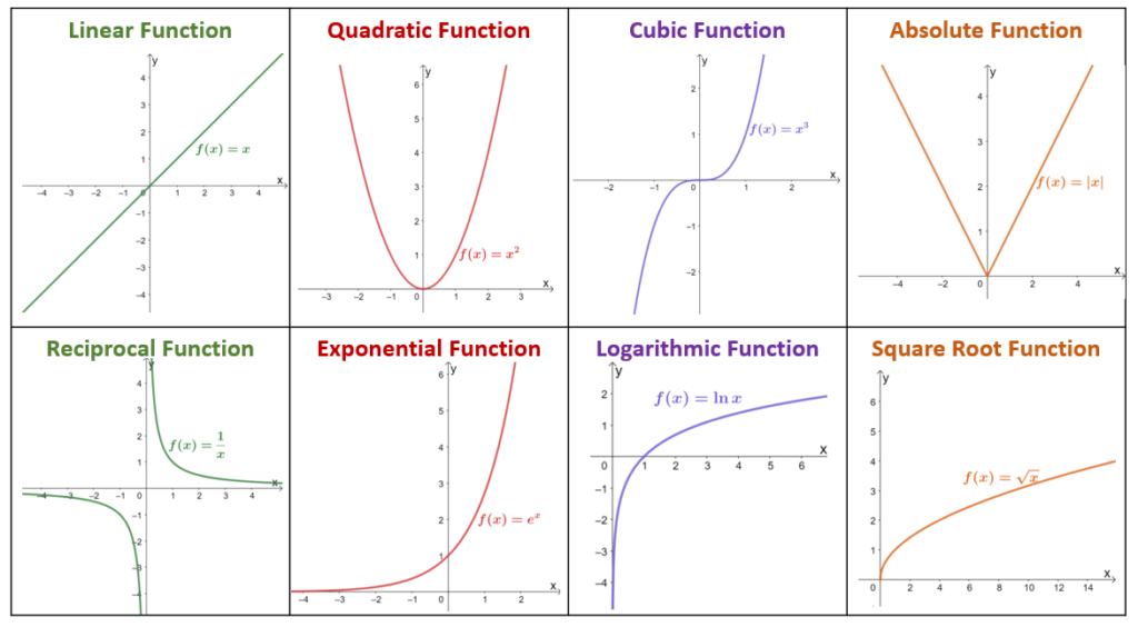
In the next part of our discussion, you’ll learn some interesting characteristics and behaviors of these eight parent functions. By knowing their important components, you can easily identify parent functions and classify functions based on their parent functions. You’ve been introduced to the first parent function, the linear function, so let’s begin by understanding the different properties of a linear function.
Linear Function
As we have learned earlier, the linear function’s parent function is the function defined by the equation, [kate]y = x[/katex] or [kate]f(x) = x[/katex]. All linear functions defined by the equation, [katex]y= mx+ b[/katex], will have linear graphs similar to the parent function’s graph shown below.

For linear functions, the domain and range of the function will always be all real numbers (or [katex](-\infty, \infty)[/katex]). The parent function passes through the origin while the rest from the family of linear functions will depend on the transformations performed on the functions.
Quadratic Function
The parent function of all quadratic functions has an equation of [katex]y = x^2[/katex]. All quadratic functions have parabolas (U-shaped curves) as graphs, so its parent function is a parabola passing through the origin as well.

By looking at the graph of the parent function, the domain of the parent function will also cover all real numbers. The vertex of the parent function lies on the origin and this also indicates the range of [katex]y =x^2[/katex]: [katex]y \geq 0[/katex] or [katex][0, \infty)[/katex]. The equation and graph of any quadratic function will depend on transforming the parent function’s equation or graph.
Cubic Function
Similarly, the cubic function’s parent function is defined by the equation, [katex]y =x^3[/katex], and also passes through the origin, [katex](0,0)[/katex]. The cubic function’s function is increasing throughout its interval. When[katex]x < 0[/katex], the parent function returns negative values. Meanwhile, the parent function returns positive values when [katex]x >0[/katex].

The cubic function’s domain and range are both defined by the interval, [katex](-\infty, \infty)[/katex]. The parent function, [katex]y =x^3[/katex], is an odd function and symmetric with respect to the origin. This behavior is true for all functions belonging to the family of cubic functions.
Absolute Value Function
The parent function of absolute value functions exhibits the signature V-shaped curve when graphed on the xy-plane. The most fundamental expression of an absolute value function is simply the parent function’s expression, [katex]y = |x|[/katex].

For the absolute value function’s parent function, the curve will never go below the x-axis. That is because the function, [katex]y = |x|[/katex] returns the absolute value (which is always positive) of the input value. This lead the parent function to have a domain of [katex](-\infty, \infty)[/katex] and a range of [katex][0,\infty)[/katex]. Absolute functions transformed will have a general form of [katex]y = a|x – h| +k[/katex] – functions of these forms are considered “children” of the parent function, [katex]y =|x|[/katex].
Reciprocal Function
From the name of the function, a reciprocal function is defined by another function’s multiplicative inverse. This means that [katex]f(x) = \dfrac{1}{x}[/katex] is the result of taking the inverse of another function, [katex]y = x[/katex].

The asymptotes of a reciprocal function’s parent function is at [katex]y = 0[/katex] and [katex]x =0[/katex]. This means that the domain and range of the reciprocal function are both
[katex](-\infty, 0) \cup (0, \infty)[/katex]
Exponential Function
An exponential function has the variable in its exponent while the function’s base is a constant. This means that there are different parent functions of exponential functions and can be defined by the function, [katex]y = b^x[/katex].
One of the most known functions is the exponential function with a natural base, e, where [katex]e \approx 2.718[/katex]. This means that this exponential function’s parent function is [katex]y = e^x[/katex].

The exponential function’s parent function is strictly increasing and normally has a horizontal asymptote at [katex]y =0[/katex]. Any parent function of the form [katex]y = b^x[/katex] will have a y-intercept at [katex](0, 1)[/katex]. Exponential function’s parent functions will each have a domain of all real numbers and a restricted range of [katex](0, \infty)[/katex].
Logarithmic Function
Similar to exponential functions, there are different parent functions for logarithmic functions. Each parent function will have a form of [katex]y = \log_a x[/katex]. This means that the parent function for the natural logarithmic function (logarithmic function with a base of e) is equal to [katex]y = \ln x[/katex].

Logarithmic functions’ parents will always have a vertical asymptote of [katex]x =0[/katex] and an x-intercept of [katex](1, 0)[/katex]. By observing the graphs of the exponential and logarithmic functions, we can see how closely related the two functions are. For logarithmic functions, their parent functions will have no restrictions for their range but their domain is restricted at [katex](0, \infty)[/katex].
Square Root Function
The square root function is one of the most common radical functions, where its graph looks similar to a logarithmic function. Its parent function will be the most fundamental form of the function and represented by the equation, [katex]y =\sqrt{x}[/katex].

Since we’re working with square roots, the square root function’s parent function will have a domain restricted by the interval, [katex](0, \infty)[/katex]. The parent function will pass through the origin. This can be used as the starting point of the square root function, so the transformation done on the parent function will be reflected by the new position of the “starting point”.
Now that we’ve shown you the common parent functions you will encounter in math, use their features, behaviors, and key values to identify the parent function of a given function. Use what you’ve just learned to identify the parent functions shown below.
Problem 1
The graphs of the functions are given as shown below. What are their respective parent functions?

Let’s take a look at the first graph that exhibits a U shape curve. This graph tells us that the function it represents could be a quadratic function. From the parent functions that we’ve learned just now, this means that the parent function of (a) is [katex]\boldsymbol{y =x^2}[/katex].
For the second graph, take a look at the vertical asymptote present at [katex]x = -4[/katex]. In addition, the function’s curve is increasing and looks like the logarithmic and square root functions. Square root functions are restricted at the positive side of the graph, so this rules it out as an option. Hence, (b) is a logarithmic function with a parent function of [katex]\boldsymbol{y =\log_a x}[/katex].
The third graph is an increasing function where [katex]y <0[/katex] when [katex]x<0[/katex] and [katex]y > 0[/katex] when [katex]x > 0[/katex]. The shape of the graph also gives you an idea of the kind of function it represents, so it’s safe to say that the graph represents a cubic function. This means that the parent function of (c) is equal to [katex]y = x^3[/katex].
Now that you’ve tried identifying different functions’ parent functions, it’s time to learn how to graph and transform different functions. The next section shows you how helpful parent functions are in graphing the curves of different functions.
How To Transform Parent Functions?
When transforming parent functions, focus on the key features of the function and see how they behave after applying the necessary transformations. All functions belonging to one family share the same parent function, so they are simply the result of transforming the respective parent function. These are the common transformations performed on a parent function:
- Vertical and horizontal translations
- Reflection over the x or y axis and both
- Vertical and horizontal stretch
- Vertical and horizontal compression
By transforming parent functions, you can now easily graph any function that belong within the same family. Let us study some examples of these transformations to help you refresh your knowledge!
Vertical and Horizontal Translations
When vertically or horizontally translating a graph, we simply “slide” the graph along the y-axis or the x-axis, respectively. This means that we can translate parent functions upward, downward, sideward, or a combination of the three to find the graphs of other child functions.
Observe the horizontal or vertical translations performed on the parent function, [katex]y =x^2[/katex].
- When [katex]y =x^2[/katex] is translated 4 units to the left or 4 units to the right, the resulting function is [katex]h(x) = (x + 4)^2[/katex] or [katex]g(x) = (x – 4)^2[/katex], respectively.
- Similarly, when the parent functions is translated 2 units upward or downward, the resulting function becomes [katex]n(x) = x^2 + 2[/katex] or [katex]m(x) =x^2 -2[/katex], respectively.
Summarize your observations and you should have a similar set to the ones shown in the table below.
| Horizontal Translations | [katex]f(x – h)[/katex] | h units to the right |
| [katex]f(x + h)[/katex] | h units to the left | |
| Vertical Translations | [katex]f(x) – k[/katex] | k units downward |
| [katex]f(x) + k[/katex] | k units upward |
Reflection Over the x-axis and the y-axis
When reflecting a parent function over the x-axis or the y-axis, we simply flip the graph with respect to the line of reflection. When reflecting over the x-axis, all the output values’ signs are reversed. Meanwhile, when we reflect the parent function over the y-axis, we simply reverse the signs of the input values.

Take a look at how the parent function, [katex]f(x) = \ln x[/katex] is reflected over the x-axis and y-axis. The function, [katex]h(x) = \ln (-x)[/katex], is the result of reflecting its parent function over the y-axis. Meanwhile, when we reflect the parent function over the x-axis, the result is [katex]g(x) = -\ln x[/katex]. This flips the parent function’s curve over the horizontal line representing [katex]y = 0[/katex].
| Reflection over the x-axis: [katex]f(x) \rightarrow -f(x)[/katex] | Reflection over the y-axis: [katex]f(x) \rightarrow f(-x)[/katex] |
Stretch and Compression of a Parent Function
When stretching or compressing a parent function, either multiply its input or its output value by a scale factor. For vertical stretch and compression, multiply the function by a scale factor, a. Meanwhile, for horizontal stretch and compression, multiply the input value, x, by a scale factor of a. Take a look at the graphs shown below to understand how different scale factors after the parent function.

By observing the effect of the parent function, [katex]y = |x|[/katex], by scale factors greater than and less than 1, you’ll observe the general rules shown below.
| Vertical Stretch | [katex]|a| >1[/katex] | Compresses the function to [katex]f(x) \rightarrow a \cdot f(x)[/katex] |
| Vertical Compression | [katex]0<|a|<1 [/katex] | Stretches the function to [katex]f(x) \rightarrow a \cdot f(x)[/katex] |
| Horizontal Compression | [katex]|a| >1[/katex] | Compresses the function to [katex]f(x) \rightarrow f(a \cdot x)[/katex] |
| Horizontal Stretch | [katex]0<|a|<1 [/katex] | Stretches the function to [katex]f(x) \rightarrow f(a \cdot x)[/katex] |
These are the transformations that you can perform on a parent function. You can combine these transformations to form even more complex functions. Don’t worry, you have a chance to test your understanding and knowledge of transforming parent functions in the next problems!
Problem 2
Transform the graph of the parent function, [katex]y = x^3[/katex], to graph the curve of the function, [katex]g(x) = 2(x -1)^3[/katex].
When transforming parent functions to graph a child function, it’s important to identify the transformations performed on the parent function.
[katex]x^3 \rightarrow (x -1)^3 \rightarrow 2(x -1)^3[/katex]
From the input value, we can see that [katex]y =x^3[/katex] is translated 1 unit to the right. Now, we can see a scale factor of 2 before the function, so [katex](x – 1)^3[/katex] is vertically compressed by a scaled factor of 2.
This means that by transforming the parent function, we have easily graphed a more complex function such as [katex]g(x) = 2(x -1)^3[/katex].
Problem 3
Transform the graph of the parent function, [katex]y = x^2[/katex], to graph the function, [katex]h(x) = 4x^2 – 3[/katex].
Similar with the previous problem, let’s see how [katex]y = x^2[/katex] has been transformed so that it becomes [katex]h(x) = \frac{1}{2}x^2 – 3[/katex].
- Apply a vertical compression on the function by a scale factor of 1/2.
- Translate the resulting curve 3 units downward.
Hence, we have the graph of a more complex function by transforming a given parent function.